Kullback-Leibler divergence asymmetry

by benmoran

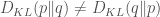
It’s widely known that the KL divergence is not symmetric, i.e.

$\displaystyle D_{KL}(p\Vert q) \neq D_{KL}(q \Vert p)$

But what’s the intuitive picture of how the symmetry fails? Recently I saw Will Penny explain this (at the Free Energy Principle workshop, of which hopefully more later). I am going to “borrow” very liberally from his talk. I think he also mentioned that he was using slides from Chris Bishop’s book, so this material might be well known from there (I haven’t read it).

f <- function(x) { dnorm(x, mean=0, sd=0.5) };
g <- function(x) { dnorm(x, mean=3, sd=2) };
curve(f(x),-6,6, col="red", ylim=c(-1,1));
curve(g(x),-6,6, col="blue", add=T);
scale <- 0.05;
curve( scale*(log(f(x))-log(g(x))),-6,6, col="red", lty=3, add=T);
curve( scale*(log(g(x))-log(f(x))),-6,6, col="blue", lty=3, add=T);

The plot shows two Gaussians, a lower variance distribution $f$ in red and a wider distribution $g$ in blue. You can also see the (scaled) quantity $\log(\frac{f}{g}) = -\log(\frac{g}{f})$ in red, and its inverse in blue.

The KL divergence $D_{KL}(f\Vert g)$ is the expectation under the red pdf of the red dotted line, and $D_{KL}(g\Vert f)$ is the corresponding expectation for the blue pair. A couple of observations reveal two sources of disagreement between them:

The KL from $f$ gives little weight to discrepancies outside the narrow region where it has the most probability density; what the broader density $g$ does out here will affect it very little
The quantity inside the expectations, the difference of logs, is actually anti-symmetric. (Somehow it’s remarkable that we can take two differently positively weighted sums of the same quantity with and without a minus sign, but always guarantee a positive result, since $D_{KL}\geq 0$ !)

Consequences for optimization

Say we have a multi-modal distribution $p$ , like this mixture of two Gaussians:

mu1 <- 4.0;
sd1 <- 0.8;
mu2 <- 1;
sd2 <- 0.5;
curve(0.5*dnorm(x, mean=mu1, sd=sd1) + 0.5*dnorm(x, mean=mu2, sd=sd2),-6,6);

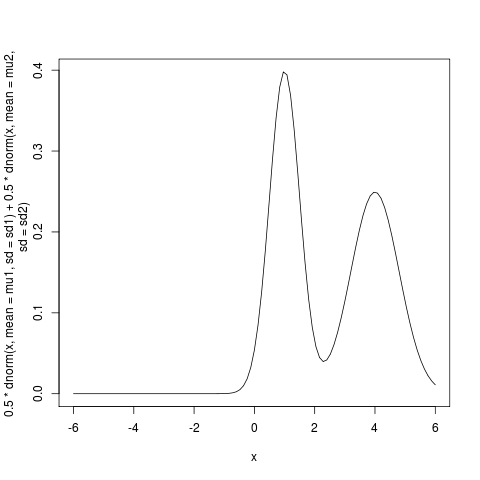
and want to approximate it with a simpler distribution $q$ – we’ll use a single Gaussian – by minimizing the KL divergence.

We can choose to minimize either $D_{KL}(q\Vert p)$ or $D_{KL}(p \Vert q)$ . Penny’s claim is that:

minimizing $D_{KL}(q\Vert p)$ results in matching a Gaussian to one of the modes (the approximating distribution is more compact than the true distribution)
minimizing $D_{KL}(p\Vert q)$ results in matching moments (our approximating distribution will have the same mean and variance as the mixture, so will be more spread out than either of the two peaks in the true distributions).

In the first case, the approximating density $q$ can choose to “ignore” troublesome parts of the target density $p$ which are difficult to fit by reducing its variance. We’ve seen above that the tails will receive little weight and can’t affect the divergence much.

In the second case, the expectation is taken under the target density $p$ , so $q$ has to try to accommodate the whole thing as best it can, multi modes and all.

(Once again David MacKay’s wonderful ITILA book has some interesting material related to this; Chapter 33 on variational free energy minimization.)

I wanted to try this optimization out. The KL divergence between two Gaussians has a closed form but it seems this is not the case for mixtures of Gaussians. So let’s fake it by sampling our densities and using discrete distributions:

xx <- -1000:1000/100;
p <- dmog(xx,4,0.8,1,0.5);

dmog <- function(x, mu1, sd1, mu2, sd2) {
  0.5*dnorm(x, mean=mu1, sd=sd1) + 0.5*dnorm(x, mean=mu2, sd=sd2);
}

kl.div <- function(p, q) {
  p %*% log(p/q);
}

dkl.pq <- function(pars) {
  q <- dnorm(xx, mean=pars[1], sd=pars[2]);
  kl.div(p, q);
}

dkl.qp <- function(pars) {
  q <- dnorm(xx, mean=pars[1], sd=pars[2]);
  kl.div(q, p);
}
init <- c(0,2);
result.qp <- optim(init, dkl.qp);
result.pq <- optim(init, dkl.pq);
plot(xx, p, type="l", col="red", ylim=c(0,1));
curve(dnorm(x, mean=result.qp$par[1], sd=result.qp$par[2]), -10,10,col="blue",add=T)
curve(dnorm(x, mean=result.pq$par[1], sd=result.pq$par[2]), -10,10,col="green",add=T)
result.qp
result.pq

We get the expected result:

the green curve is the minimum $D_{KL}(p\Vert q)$ fit, which approximate the mixture distribution’s mean (and variance?)
the blue curve is the minimum $D_{KL}(q \Vert p)$ fit, which here approximately fits the mean and sd of one of the two mixture components ( $\mu \approx 1$ , $\sigma \approx 0.5$ ). It’s a bit more touchy though, and depends on the initial conditions now.

UPDATE:

After I posted this Iain Murray linked to some nice further material on Twitter:

This note describing in more detail when the “ $D_{KL}(q\Vert p)$ is more compact” property does and doesn’t apply
A set of video lectures by David MacKay to accompany the ITILA book

In particular Lecture 14, on approximating distributions by variational free energy minimization, covers much of this material.

It also sets the mathematical scene for what I’m intending to talk about next: Karl Friston’s Free Energy Principle, which applies extensions of these ideas to understanding the brain and behaviour.

2 Comments to “Kullback-Leibler divergence asymmetry”

headbirths says:

April 29, 2013 at 9:16 pm

Hi. Nice blog, but what happened with Free Energy? I was interested in hearing your take on it.

- benmoran says:
  
  April 30, 2013 at 7:19 am
  
  Life got in the way of good intentions for my free energy blog, I must get on with it. I see you have written some posts on the subject, I’ll have a look. Thanks!

Ben Moran